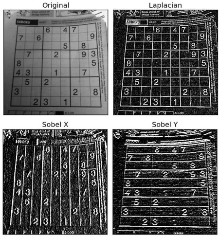
Image Gradients

Image Gradients

Goals

In this topic we will learn:

Image gradients and edge finding
And these functions: cv2.Sobel(), cv2.Scharr(), cv2.Laplacian(), etc.

Theory

OpenCV provides three types of gradient filters or high-pass filters. We will see each of them.

1. Sobel and Scharr Derivatives

Sobel operations are a joint Gaussian smoothing plus differentiation operation, so it is more resistant to noise.

You can specify the direction of the derivative to be taken, vertical or horizontal ( as arguments, yorder and xorder respectively )

You can also specify the kernel size by the argument ksize. If ksize = -1, a 3x3 Scharr filter is used instead which gives better results than a 3x3 Sobel filter.

Please refer to the docs for the kernels used.

2. Laplacian Derivatives

It calculates the Laplacian of the image given by the relation: $$\Delta src = \frac{\partial ^2{src}}{\partial x^2} + \frac{\partial ^2{src}}{\partial y^2}$$ Each derivative is found using Sobel derivatives. If ksize = 1 ( if ksize is 1 ), then the following kernel is used for filtering:

Code

The code below shows all operators in a single diagram. All kernels are of 5x5 size. Depth of output image is passed -1 to get the result in np.uint8 type.

All kernels are of 5x5 size. Depth of output image is passed -1 to get the result in np.uint8 type.

import cv2
import numpy as np
from matplotlib import pyplot as plt
img = cv2.imread('dave.jpg',0)
laplacian = cv2.Laplacian(img,cv2.CV_64F)
sobelx = cv2.Sobel(img,cv2.CV_64F,1,0,ksize=5)
sobely = cv2.Sobel(img,cv2.CV_64F,0,1,ksize=5)
plt.subplot(2,2,1),plt.imshow(img,cmap = 'gray')
plt.title('Original'), plt.xticks([]), plt.yticks([])
plt.subplot(2,2,2),plt.imshow(laplacian,cmap = 'gray')
plt.title('Laplacian'), plt.xticks([]), plt.yticks([])
plt.subplot(2,2,3),plt.imshow(sobelx,cmap = 'gray')
plt.title('Sobel X'), plt.xticks([]), plt.yticks([])
plt.subplot(2,2,4),plt.imshow(sobely,cmap = 'gray')
plt.title('Sobel Y'), plt.xticks([]), plt.yticks([])
plt.show()

Result:

An Important Topic!

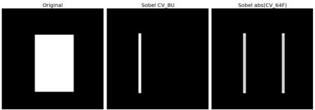
In our last example, the output datatype was cv2.CV_8U or np.uint8. But there is a small problem with this. White-to-Black transitions take a negative slope while Black-to-White transitions take a positive slope ( this is a positive value ). So when you convert data to np.uint8, all negative slopes (all slope values) are made 0.

With a simple change you can escape this edge. If you want to detect both edges, the better option is to keep output datatypes like cv2.CV_16S, cv2.CV_64F etc., take its absolute value and then convert back to cv2.CV_8U. The following code demonstrates this procedure for a horizontal Sobel filter and shows the difference in results.

import cv2
import numpy as np
from matplotlib import pyplot as plt
img = cv2.imread('box.png',0)
# Output dtype = cv2.CV_8U
sobelx8u = cv2.Sobel(img,cv2.CV_8U,1,0,ksize=5)
# Output dtype = cv2.CV_64F. Then take its absolute and convert to cv2.CV_8U
sobelx64f = cv2.Sobel(img,cv2.CV_64F,1,0,ksize=5)
abs_sobel64f = np.absolute(sobelx64f)
sobel_8u = np.uint8(abs_sobel64f)
plt.subplot(1,3,1),plt.imshow(img,cmap = 'gray')
plt.title('Original'), plt.xticks([]), plt.yticks([])
plt.subplot(1,3,2),plt.imshow(sobelx8u,cmap = 'gray')
plt.title('Sobel CV_8U'), plt.xticks([]), plt.yticks([])
plt.subplot(1,3,3),plt.imshow(sobel_8u,cmap = 'gray')
plt.title('Sobel abs(CV_64F)'), plt.xticks([]), plt.yticks([])
plt.show()