Smoothing Images

Also referred to as Smoothing Images.

Goals

• Blurring images with various low-pass filters
• Applying custom filters to images (2D Convolution)

2D Convolution ( Image Filtering )

As with one-dimensional signals, images can also be filtered with various low-pass (LPF) filters and high-pass filters (HPF) etc. A LPF helps in removing noise, or blurring the image. An HPF helps in finding edges in images.

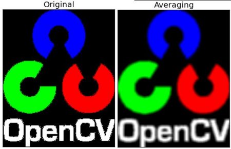
OpenCV provides a function cv2.filter2D() to convolve a kernel with an image. As an example, we will try an averaging filter on an image. A 5x5 averaging filter kernel can be defined as follows:

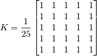
Filtering with the above kernel results in the following operation. Each pixel is averaged over a 5x5 window centered at that pixel — all pixels falling inside this window are summed and then divided by 25. This is equivalent to computing the average of pixel values inside that window. This operation is performed for all pixels of the image to produce the output filtered image. Try this code and check the result:

import cv2
import numpy as np
from matplotlib import pyplot as plt
img = cv2.imread('opencv_logo.png')
kernel = np.ones((5,5),np.float32)/25
dst = cv2.filter2D(img,-1,kernel)
plt.subplot(121),plt.imshow(img),plt.title('Original')
plt.xticks([]), plt.yticks([])
plt.subplot(122),plt.imshow(dst),plt.title('Averaging')
plt.xticks([]), plt.yticks([])
plt.show()

Result;

Image Blurring ( Image Smoothing )

Image blurring is achieved by convolving the image with a low-pass filter kernel. It is useful for removing noise. It actually removes high frequency content (e.g. noise, edges) from the image and results in edges being blurred when this filter is applied. OpenCV provides mainly four types of blurring techniques.

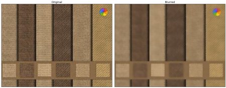
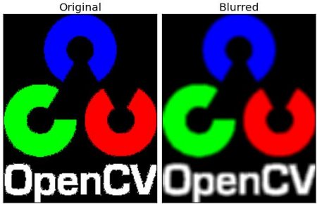
1. Averaging

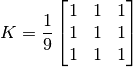
This is done by convolving the image with a normalized box filter. It simply takes the average of all the pixels under kernel area and replaces the central element. This is done by the cv2.blur() and cv2.boxFilter() functions in OpenCV. To learn more about the kernel, we should specify the width and height of the kernel. A 3x3 normalized box filter would look like this:

NOTE: If you don’t want to use a normalized box filter, use cv2.boxFilter(normalize = False).

import cv2
import numpy as np
from matplotlib import pyplot as plt
img = cv2.imread('opencv_logo.png') # read the image
blur = cv2.blur(img,(5,5)) # applied blur filter
# and output the original and new image to screen using matplotlib
plt.subplot(121),plt.imshow(img),plt.title('Original')
plt.xticks([]), plt.yticks([])
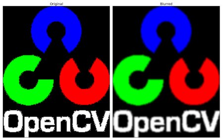
plt.subplot(122),plt.imshow(blur),plt.title('Blurred')
plt.xticks([]), plt.yticks([])
plt.show()

Result;

2. Gaussian Filtering

In this approach, instead of a box filter consisting of equal filter coefficients, a Gaussian kernel is used. This is done using the cv2.GaussianBlur() function. We should specify the width and height of the kernel which should be positive and odd. We should also specify the standard deviation in the X and Y directions, sigmaX and sigmaY respectively. If only sigmaX is specified, sigmaY is taken as equal to sigmaX. If both are given as zeros, they are calculated from the kernel size. Gaussian filtering is highly effective in removing Gaussian noise from the image. You should use the cv2.getGaussianKernel() function to do this. You can simply replace the relevant line in the code we gave above with this:

blur = cv2.GaussianBlur(img,(5,5),0)

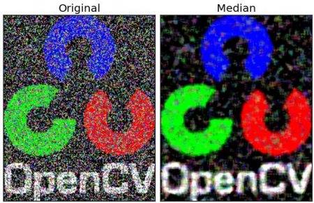
3. Median Filtering

Here, the cv2.medianBlur() function computes the median of all the pixels under the kernel window and the central pixel is replaced with this median value. This is highly effective in removing salt-and-pepper noise. One interesting thing to note is that in Gaussian and box filters, the filtered value for the central element can be a value which may not exist in the original image. However, this is not the case in median filtering, since the central element is always replaced by some pixel value in the image. This reduces noise effectively. Kernel size must be a positive odd integer.

In this demo, I added 50% noise to our original image and used a median filter. Check the result:

median = cv2.medianBlur(img,5)

4. Bilateral Filtering

As we noted, the filters we showed earlier tend to blur edges. However, that is not the case for the bilateral filter cv2.bilateralFilter(), which is highly effective in noise removal while keeping edges sharp. But the operation is slower compared to other filters.

We already saw that a Gaussian filter takes the neighbourhood around the pixel and finds its Gaussian weighted average. This Gaussian filter is a function of space alone, meaning during filtering, nearby pixels are considered. It doesn’t consider whether pixels have almost the same intensity value and it doesn’t consider whether the pixel is an edge pixel or not. The resulting effect is that Gaussian filters tend to blur edges, which is undesirable.

Bilateral filter also uses a Gaussian filter in the space domain, but it additionally uses one more (multiplicative) Gaussian filter component which is a function of pixel intensity differences. The Gaussian function of space makes sure that only nearby pixels are considered for blurring, while the Gaussian function of intensity difference (a Gaussian function of the intensity differences) ensures that only those pixels with similar intensities to the central pixel are included in blurring. So it preserves the edges since pixels at edges will have large intensity variation.

The below example demonstrates bilateral filtering (For details about the arguments, visit OpenCV docs).

blur = cv2.bilateralFilter(img,9,75,75)

Result;