· Hakan Çelik · OpenCV / Image Processing · 4 dk okuma
Morphological Transformations

Morphological Transformations
Goal
In this section,
- We will learn different morphological operations like Erosion, Dilation, Opening, Closing. ( Erosion, Dilation, Opening, Closing )
- We will see different functions like:
cv2.erode(),cv2.dilate(),cv2.morphologyEx()etc.
Theory
Morphological transformations are some simple operations based on the image shape. It is normally performed on binary images. It needs two inputs, one is our original image, the second one is called structuring element or kernel which decides the nature of the operation. Two basic morphological operators are Erosion and Dilation. Then its variant forms like Opening, Closing, Gradient etc. also come into play. We will see them one by one with help of the following image:

1. Erosion
The basic idea of erosion is just like soil erosion, it erodes away the boundaries of foreground object (Always try to keep foreground in white). So what does it do? The kernel slides through the image (as in 2D convolution). A pixel in the original image (either 1 or 0) will be considered 1 only if all the pixels under the kernel are 1, otherwise it is eroded (made to zero).
So what happens is that all the pixels near boundary will be discarded depending upon the size of the kernel. So the thickness or size of the foreground object decreases or simply the white region in the image decreases. It is useful for removing small white noises (as we have seen in the color space chapter), detaching two connected objects etc.
Here, as an example, I would use a 5x5 kernel with full of ones. Let’s see how it works:
import cv2
import numpy as np
img = cv2.imread('j.png',0)
kernel = np.ones((5,5),np.uint8)
erosion = cv2.erode(img,kernel,iterations = 1)
Result;
2. Dilation
It is just opposite of erosion. Here, a pixel element is ‘1’ if at least one pixel under the kernel is ‘1’. So it increases the white region in the image or size of foreground object increases. Normally, in cases like noise removal, erosion is followed by dilation. Because, erosion removes white noise, but it also shrinks our object. So we dilate it. Since noise is gone, they won’t come back, but our object area increases. It is also useful in joining broken parts of an object.
dilation = cv2.dilate(img,kernel,iterations = 1)
Result;

3. Opening
Opening is just another name for erosion followed by dilation. It is useful in removing noise as we explained above. Here we use the cv2.morphologyEx() function:
opening = cv2.morphologyEx(img, cv2.MORPH_OPEN, kernel)
Result:

4. Closing
Closing is reverse of Opening, Dilation followed by Erosion. It is useful in closing small holes inside the foreground objects, or small black points on the object.
closing = cv2.morphologyEx(img, cv2.MORPH_CLOSE, kernel)
Result;

5. Morphological Gradient
It is the difference between dilation and erosion of an image.
The result will look like the outline of the object.
gradient = cv2.morphologyEx(img, cv2.MORPH_GRADIENT, kernel)
Result:

6. Top Hat
It is the difference between input image and opening of the image. Below example is done for a 9x9 kernel. tophat = cv2.morphologyEx(img, cv2.MORPH_TOPHAT, kernel)
Result:

7. Black Hat
It is the difference between the closing of the input image and input image.
blackhat = cv2.morphologyEx(img, cv2.MORPH_BLACKHAT, kernel)
Result:

Structuring Element
In the previous examples we manually created a structuring element with Numpy’s help. It was rectangular in shape. But in some cases, you may need elliptical/circular shaped kernels. For this purpose, OpenCV has a function cv2.getStructuringElement(). You just pass the shape and size of the kernel, and you get the desired kernel.
# Rectangular Kernel
>>> cv2.getStructuringElement(cv2.MORPH_RECT,(5,5))
array([[1, 1, 1, 1, 1],
       [1, 1, 1, 1, 1],
       [1, 1, 1, 1, 1],
       [1, 1, 1, 1, 1],
       [1, 1, 1, 1, 1]], dtype=uint8)
# Elliptical Kernel
>>> cv2.getStructuringElement(cv2.MORPH_ELLIPSE,(5,5))
array([[0, 0, 1, 0, 0],
       [1, 1, 1, 1, 1],
       [1, 1, 1, 1, 1],
       [1, 1, 1, 1, 1],
       [0, 0, 1, 0, 0]], dtype=uint8)
# Cross-shaped Kernel
>>> cv2.getStructuringElement(cv2.MORPH_CROSS,(5,5))
array([[0, 0, 1, 0, 0],
       [0, 0, 1, 0, 0],
       [1, 1, 1, 1, 1],
       [0, 0, 1, 0, 0],
       [0, 0, 1, 0, 0]], dtype=uint8)