Canny Edge Detection

Goals

• The concept of Canny edge detection
• OpenCV function for this operation: cv2.Canny()

Theory

The Canny edge detection algorithm is a popular edge detection algorithm. It was developed by John F. Canny in 1986. It is a multi-stage algorithm and we will learn all of it.

Noise Reduction

Since edge detection is sensitive to noise in the image, the first step is to remove the noise in the image with a 5x5 Gaussian filter. We have already seen this in earlier sections.

Finding Intensity Gradient of the Image

The smoothed image is then filtered with a Sobel kernel in both horizontal direction and vertical direction to get the first derivative in horizontal and vertical directions. From these two images, we can find edge gradient and direction for each pixel as follows:

Gradient direction ( Gradient direction ) is always perpendicular to edges. It is rounded to one of four angles representing vertical, horizontal and two diagonal directions.

Non-maximum Suppression

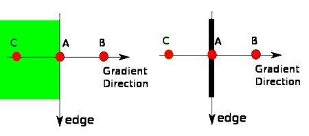
After getting gradient magnitude and direction, a full scan of image is done to remove any unwanted pixels which may not constitute the edge. For this, at every pixel, pixel is checked if it is a local maximum in its neighborhood in the direction of gradient. Check the image below:

Point A is on the edge (in vertical direction). Gradient direction is normal to the edge. Points B and C are in gradient directions. So point A is checked with points B and C to see if it forms a local maximum. If so, it is considered for next stage; otherwise, it is suppressed (put to zero). In short the result you get is a binary image with “thin edges”.

Hysteresis Thresholding

This stage decides which are all edges are really edges and which are not. For this, we need two threshold values, minVal ( minimum value ) and maxVal ( maximum value ). Any edges with intensity gradient more than maxVal ( maximum value ) are sure to be edges and those below minVal ( minimum value ) are sure to be non-edges, so discarded. Those who lie between these two thresholds are classified based on their connectivity. If they are connected to “sure-edge” pixels, they are considered to be part of edges. Otherwise, they are also discarded. See the image below.

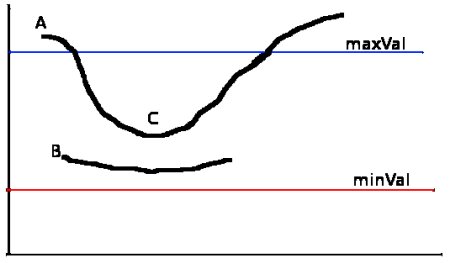
Edge A is above the maxVal, so considered as “sure-edge”. Although Edge C is below maxVal, it is connected to Edge A, so considered as valid edge and we get that full curve. But Edge B, although it is above minVal and is in same region as that of Edge C, it is not connected to any “sure-edge”, so it is discarded. Therefore it is very important that we select minVal and maxVal accordingly to get the correct result.

This stage also removes small pixel noise on the assumption that edges are long lines.

So what we finally get are strong edges in the image.

Canny Edge Detection in OpenCV

OpenCV does all the above steps described in the theory section with the cv2.Canny() function. Now we will see how to use this function.

• Our first parameter is the input argument, i.e. our image.
• The second and
• third parameters are the minimum and maximum values respectively.
• The fourth argument is aperture_size. It is the size of Sobel kernel used for finding image gradients. By default it is 3.
• The last argument is L2gradient which specifies the equation for finding gradient magnitude. If True, it uses the more accurate equation mentioned above, otherwise this function is used:

import cv2
import numpy as np
from matplotlib import pyplot as plt
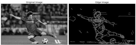
img = cv2.imread('messi5.jpg',0)
edges = cv2.Canny(img,100,200)
plt.subplot(121),plt.imshow(img,cmap = 'gray')
plt.title('Original Image'), plt.xticks([]), plt.yticks([])
plt.subplot(122),plt.imshow(edges,cmap = 'gray')
plt.title('Edge Image'), plt.xticks([]), plt.yticks([])
plt.show()

Result;